Electron Energy Loss Spectroscopy

Tools for EELS data analysis

The functions described in this chapter are only available for the EELSSpectrum class. To transform a hyperspy.api.signals.BaseSignal (or subclass) into an EELSSpectrum:

>>> s.set_signal_type("EELS")

Note these chapter discusses features that are available only for EELSSpectrum class. However, this class inherits many useful feature from its parent class that are documented in previous chapters.

Elemental composition of the sample

It can be useful to define the elemental composition of the sample for archiving purposes or to use some feature (e.g. curve fitting) that requires this information. The elemental composition of the sample can be declared using add_elements(). The information is stored in the hyperspy.api.signals.BaseSignal.metadata attribute (see eXSpy Metadata Structure). This information is saved to file when saving in the hspy format (HyperSpy’s HDF5 specification).

An utility function get_edges_near_energy() can be helpful to identify possible elements in the sample. get_edges_near_energy() returns a list of edges arranged in the order closest to the specified energy within a window, both measured in eV. The size of the window can be controlled by the argument width (default as 10)— If the specified energy is 849 eV and the width is 6 eV, it returns a list of edges with onset energy between 846 eV to 852 eV and they are arranged in the order closest to 849 eV.

>>> from hyperspy.misc.eels.tools import get_edges_near_energy
>>> get_edges_near_energy(532)
['O_K', 'Pd_M3', 'Sb_M5', 'Sb_M4']
>>> get_edges_near_energy(849, width=6)
['La_M4', 'Fe_L1']

The static method print_edges_near_energy() in EELSSpectrum will print out a table containing more information about the edges.

>>> s = hs.datasets.artificial_data.get_core_loss_eels_signal()
>>> s.print_edges_near_energy(401, width=20)
+-------+-------------------+-----------+-----------------------------+
|  edge | onset energy (eV) | relevance |         description         |
+-------+-------------------+-----------+-----------------------------+
|  N_K  |       401.0       |   Major   |         Abrupt onset        |
| Sc_L3 |       402.0       |   Major   | Sharp peak. Delayed maximum |
| Cd_M5 |       404.0       |   Major   |       Delayed maximum       |
| Sc_L2 |       407.0       |   Major   | Sharp peak. Delayed maximum |
| Mo_M2 |       410.0       |   Minor   |          Sharp peak         |
| Mo_M3 |       392.0       |   Minor   |          Sharp peak         |
| Cd_M4 |       411.0       |   Major   |       Delayed maximum       |
+-------+-------------------+-----------+-----------------------------+

The method edges_at_energy() allows inspecting different sections of the signal for interactive edge identification (the default). A region can be selected by dragging the mouse across the signal and after clicking the Update button, edges with onset energies within the selected energy range will be displayed. By toggling the edge buttons, it will put or remove the corresponding edges on the signal. When the Complementary edge box is ticked, edges outside the selected range with the same element of edges within the selected energy range will be shown as well to aid identification of edges.

>>> s = hs.datasets.artificial_data.get_core_loss_eels_signal()
>>> s.edges_at_energy()

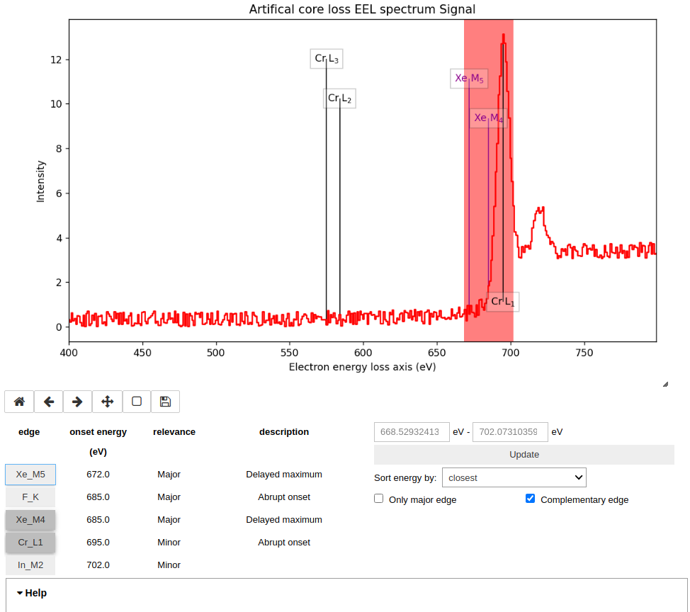
Labels of edges can be put or removed by toggling the edge buttons.

Thickness estimation

Added in version 1.6: Option to compute the absolute thickness, including the angular corrections and mean free path estimation.

The estimate_thickness() method can estimate the thickness from a low-loss EELS spectrum using the log-ratio method. If the beam energy, collection angle, convergence angle and sample density are known, the absolute thickness is computed using the method in [Iakoubovskii2008]. This includes the estimation of the inelastic mean free path (iMFP). For more accurate results, it is possible to input the iMFP of the material if known. If the density and/or the iMFP are not known, the output is the thickness relative to the (unknown) iMFP without any angular corrections.

Zero-loss peak centre and alignment

The estimate_zero_loss_peak_centre() can be used to estimate the position of the zero-loss peak (ZLP). The method assumes that the ZLP is the most intense feature in the spectra. For a more general approach see hyperspy.api.signals.Signal1D.find_peaks1D_ohaver().

The align_zero_loss_peak() can align the ZLP with subpixel accuracy. It is more robust and easy to use for the task than hyperspy.api.signals.Signal1D.align1D(). Note that it is possible to apply the same alignment to other spectra using the also_align argument. This can be useful e.g. to align core-loss spectra acquired quasi-simultaneously. If there are other features in the low loss signal which are more intense than the ZLP, the signal_range argument can narrow down the energy range for searching for the ZLP.

Deconvolutions

Three deconvolution methods are currently available:

• fourier_log_deconvolution()

• fourier_ratio_deconvolution()

• richardson_lucy_deconvolution()

Estimate elastic scattering intensity

The estimate_elastic_scattering_intensity() can be used to calculate the integral of the zero loss peak (elastic intensity) from EELS low-loss spectra containing the zero loss peak using the (rudimentary) threshold method. The threshold can be global or spectrum-wise. If no threshold is provided it is automatically calculated using estimate_elastic_scattering_threshold() with default values.

estimate_elastic_scattering_threshold() can be used to calculate separation point between elastic and inelastic scattering on EELS low-loss spectra. This algorithm calculates the derivative of the signal and assigns the inflexion point to the first point below a certain tolerance. This tolerance value can be set using the tol keyword. Currently, the method uses smoothing to reduce the impact of the noise in the measure. The number of points used for the smoothing window can be specified by the `npoints keyword.

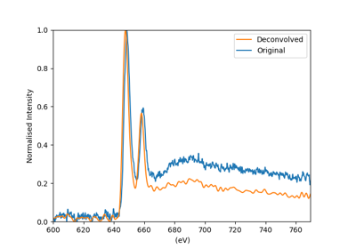
Kramers-Kronig Analysis

The single-scattering EEL spectrum is approximately related to the complex permittivity of the sample and can be estimated by Kramers-Kronig analysis. The kramers_kronig_analysis() method implements the Kramers-Kronig FFT method as in [Egerton2011] to estimate the complex dielectric function from a low-loss EELS spectrum. In addition, it can estimate the thickness if the refractive index is known and approximately correct for surface plasmon excitations in layers.

EELS curve fitting

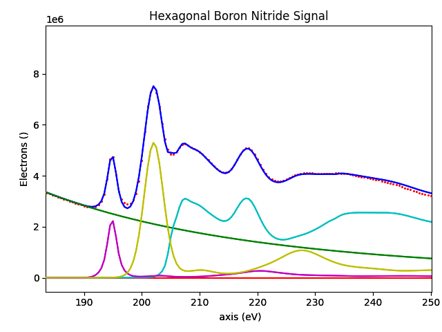
HyperSpy makes it really easy to quantify EELS core-loss spectra by curve fitting as it is shown in the next example of quantification of a boron nitride EELS spectrum from the EELS Data Base (see Loading example data and data from online databases).

Load the core-loss and low-loss spectra

>>> s = exspy.data.eelsdb(title="Hexagonal Boron Nitride",
...                       spectrum_type="coreloss")[0]
>>> ll = exspy.data.eelsdb(title="Hexagonal Boron Nitride",
...                        spectrum_type="lowloss")[0]

Creating model

Before creating a model, it is necessary to set some important experimental information, such as the beam energy and experimental angles:

>>> s.set_microscope_parameters(beam_energy=300,
...                             convergence_angle=0.2,
...                             collection_angle=2.55)

Warning

convergence_angle and collection_angle are actually semi-angles and are given in mrad. beam_energy is in keV.

Define the chemical composition of the sample, that will be used in the model:

>>> s.add_elements(('B', 'N'))

It is worth noting that in this case the experimental parameters and the list of elements are actually automatically imported from the EELS Data Base. However, with real life data, these must often be added by hand.

In order to include the effect of plural scattering, the model is convolved with the low-loss spectrum in which case the low-loss spectrum needs to be provided to create_model():

>>> m = s.create_model(ll=ll)

HyperSpy has created the model and configured it automatically:

>>> m.components
   # |       Attribute Name |       Component Name |       Component Type
---- | -------------------- | -------------------- | --------------------
   0 |             PowerLaw |             PowerLaw |             PowerLaw
   1 |                  N_K |                  N_K |           EELSCLEdge
   2 |                  B_K |                  B_K |           EELSCLEdge

Conveniently, all the EELS core-loss components of the added elements are added automatically, named after its element symbol:

>>> m.components.N_K
<N_K (EELSCLEdge component)>
>>> m.components.B_K
<B_K (EELSCLEdge component)>

Generalised Oscillator Strengths

Fitting EELS edges requires a model for the so-called Generalised Oscillator Strengths (GOS). In this example, both edges shown are K Edges, which can be fitted using an analytical model for the GOS. Fitting L edge gives more accurate results using tabulated GOS data, while for M, N and O edges the tabulated sets are strictly necessary. Therefore, tabulated data will be used by default.

The model for the GOS can be specified with the GOS argument - see create_model() for more details.

By default, a freely usable tabulated dataset, in gosh format, is downloaded from Zenodo: doi:10.5281/zenodo.7645765.

Custom GOS saved in the gosh format can be used, the following example download a previous version (1.0) of the GOS file from Zenodo (doi:10.5281/zenodo.6599071) using pooch:

>>> import pooch
>>> GOSH10 = pooch.retrieve(
...     url="doi:10.5281/zenodo.6599071/Segger_Guzzinati_Kohl_1.0.0.gos",
...     known_hash="md5:d65d5c23142532fde0a80e160ab51574",
... )
>>> m = s.create_model(gos_file_path=GOSH10)

Fitting model

By default the fine structure features are disabled. We must enable them to accurately fit this spectrum:

>>> m.enable_fine_structure()

We use smart_fit() instead of the standard fit method because smart_fit() is optimized to fit EELS core-loss spectra

>>> m.smart_fit()

This fit can also be applied over the entire signal to fit a whole spectrum image

>>> m.multifit(kind='smart')

Note

smart_fit() and m.multifit(kind='smart') are methods specific to the EELS model. The fitting procedure acts in an iterative manner along the energy-loss-axis. First it fits only the background up to the first edge. It continues by deactivating all edges except the first one, then performs the fit. Then it only activates the the first two, fits, and repeats this until all edges are fitted simultaneously.

Other, non-EELSCLEdge components, are never deactivated, and fitted on every iteration.

Print the result of the fit

>>> m.quantify()
Absolute quantification:
Elem.       Intensity
B   0.045648
N   0.048061

Visualize the result

>>> m.plot()

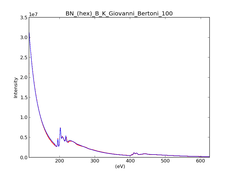
Curve fitting quantification of a boron nitride EELS core-loss spectrum from the EELS Data Base.

There are several methods that are only available in EELSModel:

• smart_fit() is a fit method that is more robust than the standard routine when fitting EELS data.

• quantify() prints the intensity at the current locations of all the EELS ionisation edges in the model.

• remove_fine_structure_data() removes the fine structure spectral data range (as defined by the fine_structure_width ionisation edge components. It is specially useful when fitting without convolving with a zero-loss peak.

The following methods permit to easily enable/disable background and ionisation edge components:

• enable_edges()

• enable_background()

• disable_background()

• enable_fine_structure()

• disable_fine_structure()

The following methods permit to easily enable/disable several ionisation edge functionalities:

• set_all_edges_intensities_positive()

• unset_all_edges_intensities_positive()

• enable_free_onset_energy()

• disable_free_onset_energy()

• fix_edges()

• free_edges()

• fix_fine_structure()

• free_fine_structure()

Fine structure analysis

The fine structure of an EELS ionization edge manifests as distinct features within the first few tens of eVs energy. It is due to variations in the electron’s energy loss probability caused by the interactions with the material’s electronic structure. It offers insights into the material’s electronic properties, bonding, and local environments. Therefore, we cannot model them from first-principles because i) the material is usually unknown ii) HyperSpy only supports Hydrogenic and Hartree-Slater EELS core-loss models. Instead, the EELSCLEdge component includes features for EELS fine structure modelling and analysis using functions to mimic the fine structure features. The most basic consists in modelling the fine structure of ionization edges using a spline function. You can activate this feature by setting the fine_structure_active attribute of a given EELSCLEdge component to True. For example:

>>> m.components.N_K.fine_structure_active = True

To enable the fine structure component for all or a selection of ionization edges, you can use the enable_fine_structure() method:

>>> m.enable_fine_structure()

The width of the fine structure (i.e., the region of the ionization edge that we will model using a spline instead of the atomic simulation) can be defined using the fine_structure_width attribute. It defaults to 30 eV. Another important parameter is the fine_structure_smoothing. It takes a value between 0 and 1, 0.3 by default. Decreasing it makes the spline smoother, at the expense of detail. The optimal value should reproduce well the fine structure features but not the noise.

The parameters controlling the shape of the spline function are stored in the fine_structure_coeff attribute. Notice that the value of the component.Parameter is a tuple that contains a list of float. Its length depends on the value of fine_structure_width and fine_structure_smoothing, and it will be reset to 0 when any of those values change.

If we zoom-in the fine structure region of the Boron-K ionization edge of the BN model above, we notice that the fit is actually not very good:

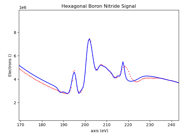
Boron-K EELS ionization edge fine structure model using default values

Let’s try to improve the fine structure model of the Boron-K and Nitrogen-K ionization edges by:

• Adjusting the position of the B-K edge onset to match the experimental spectrum

• Adjusting the width of the fine structure

>>> m.set_signal_range(160.)
>>> m.components.B_K.onset_energy.value = 194
>>> m.components.N_K.onset_energy.value = 402.5
>>> m.components.B_K.fine_structure_width = 40
>>> m.components.N_K.fine_structure_width = 45
>>> m.components.B_K.fine_structure_smoothing = 0.4
>>> m.smart_fit()

After executing the commands above, the model of the fine structure of both edges is much better, and the B/N ratio gets closer to one. Indeed, when performing EELS quantification using the low-loss region to account for multiple scattering, improving the model of the fine structure is essential to obtain an accurate parameter estimation.

When fitting edges with fine structure enabled, it is often desirable that the fine structure region of nearby ionization edges does not overlap. HyperSpy provides a method, resolve_fine_structure(), to automatically adjust the fine structure to avoid overlap. This method is executed automatically when e.g. components are added or removed from the model, but sometimes is necessary to call it manually.

Sometimes it is desirable to disable the automatic adjustment of the fine structure width. It is possible to suspend this feature by calling suspend_auto_fine_structure_width(). To resume it use suspend_auto_fine_structure_width()

Fine structure analysis

Fine structure analysis consists on measuring different features of the fine structure (e.g., peak position, area, …). Often, these features can be related to the ionized atom environment. For this purpose, we need to replace the spline function, that we have used so far to fit the fine structure, with other functions that accurately model the features that we want to measure.

As an example, lets model the first two peaks of the Boron-K edge fine structure using two Gaussian functions instead of the spline function:

>>> g1 = hs.model.components1D.GaussianHF(centre=194.7, fwhm=3., height=5)
>>> g1.name = "B_K_l1"
>>> g2 = hs.model.components1D.GaussianHF(centre=201.9, fwhm=5., height=5)
>>> g2.name = "B_K_l2"

Next, we need to let HyperSpy know that these two Gaussian functions are part of the fine structure of the Boron-K edge. Otherwise, the Gaussian functions would be added over the current spline fine structure, which is not what we want: we want to replace the spline function with the two Gaussian functions in the first 10 eV from the Boron-K ionization edge onset. For that, we simply add them to the fine_structure_components set:

>>> m.components.B_K.fine_structure_components.update((g1, g2))

Note that the Gaussian components are added to the model:

>>> m.components
# |      Attribute Name |      Component Name |      Component Type
---- | ------------------- | ------------------- | -------------------
0 |            PowerLaw |            PowerLaw |            PowerLaw
1 |                 N_K |                 N_K |          EELSCLEdge
2 |                 B_K |                 B_K |          EELSCLEdge
3 |              B_K_l1 |              B_K_l1 |          GaussianHF
4 |              B_K_l2 |              B_K_l2 |          GaussianHF

We still need to use the spline function to model the fine structure region that we are not modelling using the Gaussian functions. Therefore, we make sure that fine_structure_spline_active is True and we set its onset to around the minimum between the 2nd and 3rd (~205 eV) fine structure peaks:

>>> m.components.B_K.fine_structure_spline_active = True
>>> m.components.B_K.fine_structure_spline_onset = 205. - m.components.B_K.onset_energy.value
>>> m.smart_fit()
>>> m.plot(plot_components=True)

Boron-K EELS ionization edge fine structure model using two Gaussian functions for the first two white-lines, and a spline function for the rest of the fine structure.